
The use of pre-trained deep learning models for the photographic assessment of donor livers for transplantation

Abstract
Aim: Hepatic steatosis is a recognised major risk factor for primary graft failure in liver transplantation. In general, the global fat burden is measured by the surgeon using a visual assessment. However, this can be augmented by a histological assessment, although there is often inter-observer variation in this regard as well. In many situations the assessment of the liver relies heavily on the experience of the observer and more experienced surgeons will accept organs that more junior surgeons feel are unsuitable for transplantation. Often surgeons will err on the side of caution and not accept a liver for fear of exposing recipients to excessive risk of death.
Methods: In this study, we present the use of deep learning for the non-invasive evaluation of donor liver organs. Transfer learning, using deep learning models such as the Visual Geometry Group (VGG) Face, VGG16, Residual Neural Network 50 (ResNet50), Dense Convolutional Network 121 (DenseNet121) and MobileNet are utilised for effective pattern extraction from partial and whole liver. Classification algorithms such as Support Vector Machines, k-Nearest Neighbour, Logistic Regression, Decision Tree and Linear Discriminant Analysis are then used for the final classification to identify between acceptable or non-acceptable donor liver organs.
Results: The proposed method is distinct in that we make use of image information both from partial and whole liver. We show that common pre-trained deep learning models can be used to quantify the donor liver steatosis with an accuracy of over 92%.
Conclusion: Machine learning algorithms offer the tantalising prospect of standardising the assessment and the possibility of using more donor organs for transplantation.
Keywords
INTRODUCTION
Liver transplantation is the treatment of choice for patients with liver failure and organ confined liver tumours. Across the world, the major limiting factor for transplantation is the availability of optimal organs for transplantation. In the United Kingdom, from 2021 to 2022, 870 livers were retrieved for transplantation, but 18% were deemed unsuitable for transplantation and discarded[1]. The most common reason livers are turned down for transplantation is hepatic steatosis or "fatty liver disease". Hepatic steatosis is linked to the increasing prevalence of non-alcoholic fatty liver diseases (NAFLD)[1]. In fact, NAFLD is the most common hepatic disease in developed nations affecting more than 38% of obese children and 30% of adults[2-4]. Fatty liver disease often co-exists with diabetes and vascular disease, leading to stroke and, in some cases, brain death. Organ donors are therefore likely to have some degree of hepatic steatosis. Macrosteatosis (large droplets of fat within liver cells) is particularly associated with early liver graft failure and post-transplant death[5]. The grading of hepatic steatosis is generally on the basis of cellular distribution, with macrosteatosis being considered far more clinically significant than microsteatosis and the percentage of cellular involvement is broken down into mild (
Histopathological assessment of steatosis is considered the gold standard in many countries but is not available in the United Kingdom for most centres. A recent review highlighted the specific problems with liver biopsy in the deceased donor situation. Accurate visual estimation of hepatic steatosis is dependent on the experience of the histopathologist and often not reliable using the frozen section technique, which is the most utilised. In addition, there is both significant intra observer and inter observer variation in the assessment of a small tissue sample- which is peripheral and may not represent the full organ. The techniques are also time consuming and may lead to serious complications such as bleeding and haematoma formation[7-10]. A clinically useful assessment of fatty liver disease needs to be available at the point of organ retrieval- cheap, fast, non-invasive and correlates with real world outcomes. Ultrasound, MRI, and CT diagnostic imaging have all been trialled in this environment with limited success[2, 11-13].
It has been shown that an experienced liver transplant surgeon is as effective at visually assessing a liver graft for steatosis as an expert liver histopathologist[14]. As a result, various studies have evaluated photographic assessment combined with various automation processes as potential alternatives[9, 15] to determine whether a liver is transplantable or untransplantable based on the amount of hepatic steatosis on the liver graft using artificial intelligence techniques.
A French study[11] compared a smartphone based camera with a biopsy and donor data to characterise whether a donor liver had
Recent dramatic increases in computational capacity and the increase in data volume have led to the substantial development of machine learning techniques. As a result, attention has dramatically tilted towards the use of artificial intelligence (AI) in healthcare. Currently, deep learning models - specifically, CNNs have gained much popularity for medical image analysis due to their capability to automatically process and extract useful discriminatory features.
CNNs are configured in a way that enable them to learn distinct types of features from images. For example, the first lower layers extract low-level features such as the image textures, while the deeper layers extract high-level features that relate to the actual appearance of the input image. Several deep learning models for image classification were proposed and trained on huge image databases. However, medical image datasets are oftentimes not sufficient to develop well-functioning models from scratch. Consequently, transfer learning is applied using existing models trained on large nonmedical image databases, making some adjustments, and re-using them for the medical problem of interest. This method has been used in solving many problems in medical image analysis, such as the classification of burns[16, 17], cancer[18, 19], Covid-19[20-22], and skin lesions[23, 24].
The work we present in this paper contributes to the domain of medical image analysis in the following manner.
1. We demonstrate that pre-trained deep learning models can be successfully utilised to carry out the transplantability assessment of donor graft organs for liver transplantation using both partial (biopsied) and full liver images.
2. We show how features from pre-trained deep learning models in conjunction with common classification algorithms can be used to systematically evaluate and analyse partial and as well as full liver images.
3. We discuss a methodology for experimentation and evaluation of pre-trained deep learning models which has the potential to assist effective and consistent clinical decision making during the liver transplant pathway.
The rest of the paper is organised as follows. First, we present the materials and in-depth descriptions of the method used. Then, we present the experimental set-up and the results. Finally, we present a comprehensive discussion of the results along with an extensive performance analysis of the approach.
MATERIALS AND METHODS
Dataset
In 2001 the Birmingham and Newcastle liver transplant units collaborated to produce a joint photograph point of care system called NORIS (Newcastle Organ Retrieval Imaging System). NORIS comprised a basic laptop, modem, mobile phone and was supported by the general packet radio service (GPRS) network[25]. The software allowed only a basic assessment with no specific extra functionality. Uptake by retrieval teams was low and eventually abandoned in 2003. However, the images that were collected as part of the initial pilot did have utility for training and research purposes and formed the basis for the initial analysis as part of this study. In many ways, the idea was "ahead of its time" and the failings were due to basic technology, narrow bandwidth and poor user functionality. With 5G networks, 10MB cameras and smartphones the concept is now being re-explored by transplant teams across the globe.
All the pictures were taken on the "backtable" - a sterile surgical field area with the liver in a bowl surrounded by ice slush to keep it cool. At this stage, the majority of the blood has been washed out by organ storage solution, as you suggest and is the normal place where the surgeon would make his/her assessment as to the overall quality.
Hepatic grading
Grading of the liver steatosis is carried out using the following standard systematic scoring[9]: steatosis
Image pre-processing
The first crucial step that was applied to the dataset was pre-processing. This is important to ensure we get the best image quality by eliminating unnecessary distortions to ensure the image is upgraded to a better quality needed for further processing. Therefore, all images were segmented, removing the background effects as seen in a sample depicted in Figure 1. Specifically, colour image segmentation was used using k-means algorithm[26, 27]. Furthermore, because the images have varying sizes, we then resized them into 224
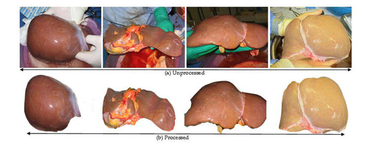
Figure 1. Samples of the pre-processed and post-processed images of liver organ.
Extraction of patch samples
Patch extraction is an effortless way of decomposing the original image into small units or segments. It allows extraction of specific target regions in an image as well as enlarging the deficient database of images to a considerable size. Here we decided to extract random pixels (regions) from each image. Two windows around different locations of the target pixels were cropped out randomly from each image. The targeted regions are fatty pixels and non-fatty (normal) pixels. In each of the classes, two random crops (patches) were extracted. 1st class (transplantable) with 836 patch images and the 2nd class (non-transplantable) with 922 patch images.
Feature extraction and classification
Images contain useful information that humans are unable to extract with their visual systems. As such, a deep neural network, an artificial subset of the human brain, is recently being used to learn such useful patterns from images. Though neural networks are more capable of learning more robustly than human, but they demand a huge amount of data for them to generalise effectively. Generally, training a neural network can be carried out in three separate ways: training from scratch, fine-tuning the existing (trained) model and using off-the-shelf neural network features. In the absence of such enormous data, a promising approach known as transfer learning is being used[16, 28, 29] which allows us to extract features. There are several pre-trained models readily available to be utilised for this, such as VGG-Face, VGG-16, ResNet-50, DenseNet121 and MobileNet.
For each of the model, an input image
At this point, it is important to also note that neural network models have two main parts: the feature extraction part and classification part. By passing the image into the network, the CNN model learns features from the initial layers and at the extreme end of the network, classification take place. The feature extraction layers learn distinctive features, some layers may be learning features such as edges, colours, and textures, while some layers may be learning some highly complex features. Therefore, knowing that each layer from the feature extraction part learns some useful information from the inputs, the classification part in each CNN model was chopped off and replaced with a new classifier. Algorithm 1 below describes the feature extraction process.
Input: Training dataset
for
for
image = read a sample image
image = segment (image)
image = resize(image)
feature = ExractFeatures(image)
normalised_feature = normalise(feature)
endfor
endfor
Algorithm 1. Algorithm describing the feature extraction process.
Feature extraction using CNN models
The CNN models used in this study for the assessment of the liver images are of 5 architectures: VGG-face[30], VGG16[31], ResNet50[32], DenseNet121[33] and MobileNet[34]. VGG-face is a CNN model trained on human face images containing 2.6 million images with over 2.6K people, each identity having 1000 samples. VGG16 was trained on ImageNet database[35], which contains more than 14 million labelled high-resolution images containing at least 22, 000 object categories. The subset of this database was used containing at least 1.2 million training images, 50, 000 and 150, 000 images for validation and testing respectively. Both VGG-face and VGG16 are of the same architecture but differ in two ways: the former was trained on face images (indirectly on one of the human organ datasets - skin) and has at least 2.6 thousand outputs (classes), while the former was trained on object categories and 1000 classes. Figure 2 below depicts the architectural illustration of VGG models.
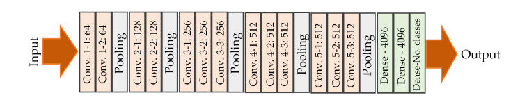
Figure 2. The architecture of the VGG model. VGG: Visual geometry group.
When the number of layers in CNN increases, the accuracy abruptly is affected or degrades, and the deep learning community wanted to have a deep network without any compromise in terms of accuracy. The ResNet50 is a deep feed forward CNN model, one of the proposed models that comes with an extra connection known as skip connection to overcome the problem. The skip connection allows transfer of input from one layer to a later layer as depicted in an illustration in Figure 3, it carries older input which serves as freshly input to the later layer.
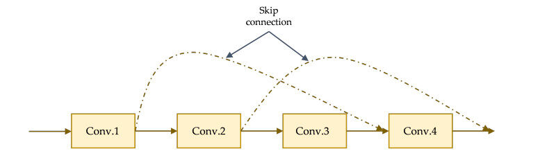
Figure 3. Illustration of the connection from the input layer to later layers.
The idea of residual mapping in the ResNet was extended in a model proposed by Huang et al. in 2016[33]. The new idea of residual mapping is propagating the output of each of the previous blocks into all subsequent block as depicted in Figure 4. Doing this kind of propagating all previous outputs. from each block into each subsequent block helps in strengthening feature transfer and solves the vanishing gradient problem. DenseNet became the winner of ImageNet Large Scale Visual Recognition Challenge (ILSVRC)-2016.
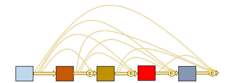
Figure 4. Illustration of the how various blocks in the model are connected.
The MobileNet was proposed by Howard et al.[34]. This model was built based on using depthwise separable convolutions, a factorised form of normal convolution by dividing the convolution operation into two; the depthwise convolution and 1
In all the 5 pre-trained CNN models described above, the classification layers were chopped off, and the remaining filtering (convolutions) layers were used for the future extraction. Then subsequently, these features were fed into each of the classification algorithms discussed in the following sub-section.
Classification of features
For the classification task, we employed five different classification algorithms: SVM, K-Nearest Neighbour (KNN), Linear Regression (LR), Decision Tree (DT) and Linear Discriminant Analysis (LDA). Classification can be restricted between two two-class problems, and the generalisation capability remain intact. In a classification problem involving two classes, the goal is to separate the two classes using a function induced from the given training examples. This will end up producing an effective classifier that will perform well on new examples.
SVM is one of those binary classifiers that operates by determining the optimal separating hyperplane between the two given classes, thereby maximising the distance (margin) between the closest point from each class[36]. Let's assume a problem is presented with set of training vectors that belongs to two separate classes,
KNN, on the other hand, is based on a distance function that determines the similarity between the two given examples[37]. The distance function which can be used to determine the similarity between the two instances is the standard Euclidean distance
LR is used to find the relationship between an independent variable (input), say
DT classification algorithm works by splitting the data repeatedly to maximise the separation of the data and eventually resulting to a tree-like form[39].
LDA is a technique commonly used for both dimensionality reduction and classification[40]. It works by outlining a decision boundary trying to separate two or multiples classes. The aim of LDA is to maximise between-class variance while minimising within-class variance.
All the classifiers were trained on each of the features from the feature extractors. During the training, the features were split into two folds: 80% for training and 20% for testing. Moreover, using the 80% split, each classifier was trained using
EXPERIMENTAL RESULTS
This section presents the experimental results. An illustration of the whole experimental procedure is depicted in Figure 5. It describes the complete process starting from the input, pre-processing (which involves segmentation of the liver images from the background and objects, rescaling the width and the height of the images, and extraction of the patch samples from each of the full liver images), the feature extraction, up to the training section of all the classifiers.
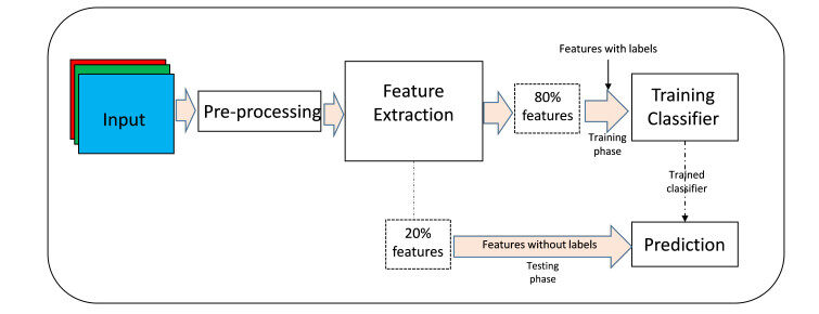
Figure 5. Illustration of the experimental procedure.
We present the results in two folds: first, the classification results from the input patch images, and secondly the classification results from the use of full liver images.
Partial liver images
Extraction of random partial liver images is obviously like histological biopsy sample extraction, where experienced histologists pinch out a small tissue from the whole liver and subsequently make the analysis visually or with the aid of a dedicated microscope. Here, the extracted patches are automatically analysed using deep learning algorithms. Table 1 shows the classification performances of each of the 5 classifiers using each of the features. For the VGGFace features, 85.42%, 82.01%, 86.55%, 78.98% and 68.37% accuracy were obtained using SVM, KNN, LR, DT and LDA classifiers, respectively. For the VGG16 features, 90.72%, 69.51%, 90.53%, 80.30% and 88.26% accuracy were obtained by SVM, KNN, LR, DT and LDA classifiers, respectively. For the ResNet50 features, 90.91%, 85.80%, 92.99%, 84.09% and 83.52% accuracy were obtained by the SVM, KNN, LR, DT and LDA classifiers, respectively. For the DenseNet121 features, 88.83%, 86.17%, 90.53%, 82.39% and 73.86% accuracy were obtained by the SVM, KNN, LR, DT and LDA classifiers, respectively. Lastly, for the MobileNet features, 72.54%, 74.24%, 76.89%, 65.72% and 60.04% accuracy were obtained by the SVM, KNN, LR, DT and LDA classifiers, respectively.
Performance accuracy (%) with patch images
| Features | Classifiers | ||||
| SVM | KNN | LR | DT | LDA | |
| SVM: Support vector machine; KNN: K-nearest neighbour; LR: linear regression; DT: decision tree; LDA: linear discriminant analysis. | |||||
| VGGFace | 85.42 | 82.01 | 86.55 | 78.98 | 68.37 |
| VGG16 | 90.72 | 69.51 | 90.53 | 80.30 | 88.26 |
| ResNet50 | 90.91 | 85.80 | 92.99 | 84.09 | 83.52 |
| DenseNet121 | 88.83 | 86.17 | 90.53 | 82.39 | 73.86 |
| MobileNet | 72.54 | 74.24 | 76.89 | 65.72 | 60.04 |
Full liver images
The result here is obtained from full liver images used as input. The classification results presented in Table 2 show that with the VGGFace features, 96.31%, 90.04%, 95.94%, 91.51% and 60.52% accuracy were obtained by the SVM, KNN, LR, DT and LDA classifiers, respectively. With the VGG16 features, 97.79%, 94.10%, 97.79%, 92.25% and 95.57% accuracy were obtained by the SVM, KNN, LR, DT and LDA classifiers, respectively. With the ResNet50 features, 97.05%, 89.67%, 97.79%, 92.99 and 92.25% accuracy were obtained by the SVM, KNN, LR, DT and LDA classifiers, respectively. With the DenseNet121 features, 99.63%, 95.94%, 99.26%, 91.88% and 89.30% accuracy were obtained by the SVM, KNN, LR, DT and LDA classifiers, respectively. Finally, with the MobileNet features, 95.57%, 94.10%, 95.57%, 91.14% and 88.19% accuracy were obtained by the SVM, KNN, LR, DT and LDA classifiers, respectively.
Performance accuracy (%) with full images
| Features | Classifiers | ||||
| SVM | KNN | LR | DT | LDA | |
| SVM: Support vector machine; KNN: K-nearest neighbour; LR: linear regression; DT: decision tree; LDA: linear discriminant analysis. | |||||
| VGGFace | 96.31 | 90.04 | 95.94 | 91.51 | 60.52 |
| VGG16 | 97.79 | 94.10 | 97.79 | 92.25 | 95.57 |
| ResNet50 | 97.05 | 89.67 | 97.79 | 92.99 | 92.25 |
| DenseNet121 | 99.63 | 95.94 | 99.26 | 91.88 | 89.30 |
| MobileNet | 95.57 | 94.10 | 95.57 | 91.14 | 88.19 |
It is obvious that performances of the classifiers as shown in Table 2 are more accurate than the results presented in Table 1. The discussion of these results is elaborated in the next section.
RESULTS AND DISCUSSIONS
Our study has shown that an AI trained algorithm can perform to the standard of experienced liver transplant surgeons in terms of hepatic steatosis assessment and organ transplantability. In this section, we analysed the results presented in the previous section, starting with the results from the patch liver image samples and then the full liver image samples.
For features from the VGGFace, the LR classifier achieved better results and effectively discriminated transplantable and non-transplantable livers with 86.55% accuracy. The worst choice is the LDA classifier which achieved an accuracy of 68.35%. For the features from the VGG16, transplantable and non-transplantable livers were effectively discriminated using the SVM classifier with an accuracy of 90.72%, while the worse scenario was by using the KNN classifier which achieved an accuracy of 69.51%. For the features from the ResNet50, an accuracy of 92.99% was obtained using the LR classifier, which recorded the best discrimination between transplantable and non-transplantable livers. The worst case is the use of the LDA classifier achieved a classification accuracy of 83.52%. For the features from the DenseNet121 and MobileNet, the LR classifier produced the best results, discriminating between transplantable and non-transplantable livers with an accuracy of 90.53% and 76.89%, respectively. Similarly, LDA failed to perform well with the DenseNet and MobileNet features and achieved accuracy of 73.86% and 60.04% respectively.
If we consider the different types of features, starting with patch liver images, the VGGFace features along with the LR classifier produced a more satisfying outcome than with any other classifier. Also, the ResNet50, DenseNet121 and MobileNet features along with LR produced better results, except the VGG16 features that produced better results with the SVM classifier. Similarly, all features along with the LDA classifier achieved less impressive outcomes except the VGG16 features along with the KNN is worst. In general, the classification of transplantable and non-transplantable livers using patch images is much more impressive with the ResNet50 features and the LR classifier, while the poorest performance is with the MobileNet features and the LDA classifier.
The results using features of full liver images, as presented in Table 2, show that features from the VGGFace and DenseNet121 performed better with the SVM classifier and worst with the LDA classifier. The performances of SVM and LR are same for both VGG16 and MobileNet features, but the VGG16 features are poor with the DT classifier while the MobileNet features are poor with the LDA classifier. The ResNet50 features worked well with the LR classifier and poor with the KNN classifier. The results show that with full liver images, it is much more effective to classifier transplantable and non-transplantable liver features with the SVM and not well enough with the LDA. In general, the DenseNet121 features, along with the SVM achieved a near perfect discrimination accuracy than all the rest of the combinations.
Moreover, from the distinct types of feature sets used, 4 of the features were obtained from the ImageNet models (model trained on a database containing non-human organ representations), but the VGGFace was trained on human faces, which indirectly implies that it was able to learn features from one of the human organs (skin). Despite such an advantage, the performances of the classifier were not better than those models trained on features from ImageNet models. This astonishing achievement of the classifiers with ImageNet features can be attributed to the fact the ImageNet models were able to learn from diverse feature representations, which makes them so strong in learning deep discriminatory patterns. This observation was also made in a study[28] where features from the ImageNet models outperformed features from the VGGFace model in the effort to discriminate between skin burns and healthy skin images.
An additional observation from the results in Tables 1 and 2, classifying the liver in its full form rather than from a random smaller portion of it yielded better accuracy. One of the problems histologists face during the analysis of biopsied samples from organs is the sampling error. The biopsied sample may not have or contain the full representation of the problem they are trying to analyse. As such, there is a high tendency to get false alarms. We attributed the mediocre performance to the fact that the random patches selected from the liver images suffered sampling errors. Utilising full images of the liver shows that the feature extractors were able to capture features from various parts of the liver and grab the discriminatory features in detail, which led to the improvement in the classification accuracy.
Performance evaluation
It is a well-known practice that before any diagnostic procedure is put into practice, it must undergo a series of checks to ascertain its ability to discriminate, say, diseased and non-diseased samples. The Receiver Operating Characteristics (ROC) curve is one of the most popular tools for evaluating diagnostics tests. It is a graphical tool based on detection probability [True Positive Rates (TPR)] versus false alarm probability [False Positive Rates (FPR)], where the area under the ROC curve (AUC) is computed and used as a diagnostic measure. The AUC value less than or equal to 0.5 represents poor measure and better when the value goes higher, with a value of 1 representing perfect diagnosis.
Figures 6-10 show the ROC curve generated on patch liver data. Figure 6 presents the ROC curve using the SVM classifier from each of the patterns. The AUCs (Area Under the Curves) are 0.8549, 0.9090, 0.9091, 0.8869, and 0.7258 are computed from VGGFace, VGG16, ResNet50, DenseNet121 and MobileNet features, respectively. The evaluation result depicted in Figure 7 shows the ROC curve using the KNN classifier generated from each feature set. The result shows the AUCs of 0.8278, 0.7189, 0.8673, 0.8665 and 0.7454 computed from VGGFace, VGG16, ResNet50, DenseNet121 and MobileNet features, respectively. With the LR classifier as depicted in Figure 8, the AUC using each of the features are 0.8670, 0.9072, 0.9306, 0.9052, and 0.7718 using VGGFace, VGG16, ResNet50, DenseNet121 and MobileNet, respectively. The best diagnostic result was obtained using ResNet50 features.
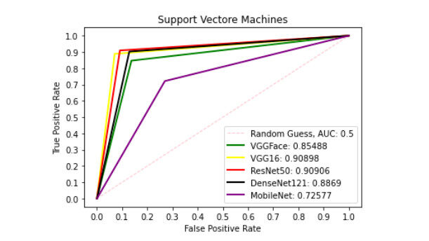
Figure 6. ROC curve with SVM comparing deep features using patch liver images. ROC: Receiver operating characteristics; SVM: support vector machine.
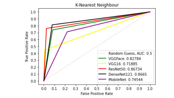
Figure 7. ROC curve with KNN comparing deep features using patch liver images. ROC: Receiver operating characteristics; KNN: K-nearest neighbour.
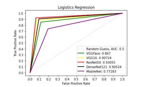
Figure 8. ROC curve with LR comparing deep features using patch liver images. ROC: Receiver operating characteristics; LR: linear regression.
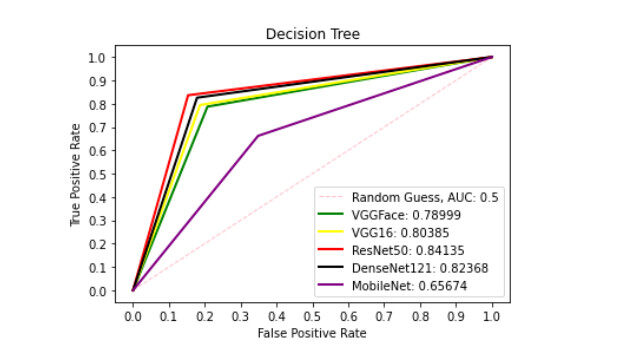
Figure 9. ROC curve with DT comparing deep features using patch liver images. ROC: Receiver operating characteristics; DT: decision tree.
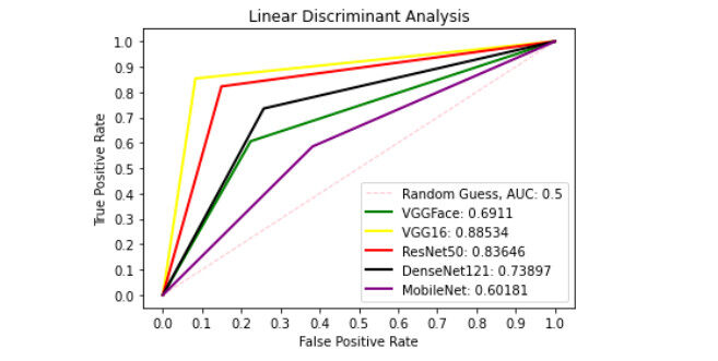
Figure 10. ROC curve with LDA comparing deep features using patch liver images. ROC: Receiver operating characteristics; LDA: linear discriminant analysis.
Figure 9 presents ROC curve with DT classifier with best AUC value of 0.8414 from ResNet50 features, 0.7900 from VGGFace features, 0.8039 from the VGG16 features, 0.8237 from the DenseNet121 features and 0.6567 from the MobileNet features. With the LDA classifier, the VGG16 features produced better performance with AUC score of 0.8853 as shown in Figure 10, 0.6911, 0.8365, 0.7390, and 0.6018 with the VGGFace, ResNet50, DenseNet121 and MobileNet, respectively. With full liver images, the SVM's performance is depicted in Figure 11 with AUC score of 0.9615, 0.9765, 0.9680, 0.9958 and 0.9530 using the VGGFace, VGG16, ResNet50, DenseNet121 and MobileNet features, respectively. With the KNN classifier, the performance is depicted in Figure 12 with AUC of 0.9079, 0.9380, 0.9066, 0.9631 and 0.9458 using the VGGFace, VGG16, ResNet50, DenseNet121 and MobileNet features, respectively. The AUC scores in Figure 13 are 0.9573, 0.9756, 0.9756, 0.9915 and 0.9530 computed from the LR classifier using the VGGFace, VGG16, ResNet50, DenseNet1321 and MobileNet features, respectively. In Addition, the AUC scores with the DT classifier as depicted in Figure 14 show 0.9132, 0.9188, 0.9302, 0.9174 and 0.9099 were obtained using features from the VGGFace, VGG16, ResNet50, DenseNet121 and MobileNet respectively Moreover, as shown in Figure 15, 0.6087, 0.9530, 0.9227, 0.8984, and 0. 8790 AUC scores were obtained using the LDA classifier with the VGGFace, VGG16, ResNet50, DenseNet121 and MobileNet features, respectively.

Figure 11. ROC curve with SVM comparing deep features using full liver images. ROC: Receiver operating characteristics; SVM: support vector machine.
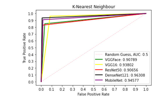
Figure 12. ROC curve with KNN comparing deep features using full liver images. ROC: Receiver operating characteristics; KNN: K-nearest neighbour.
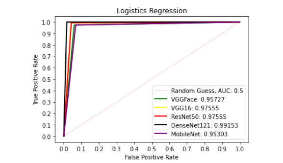
Figure 13. ROC curve with LR comparing deep features using full liver images. ROC: Receiver operating characteristics; LR: linear regression.
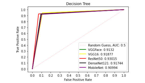
Figure 14. ROC curve with DT comparing deep features using full liver images. ROC: Receiver operating characteristics; DT: decision tree.
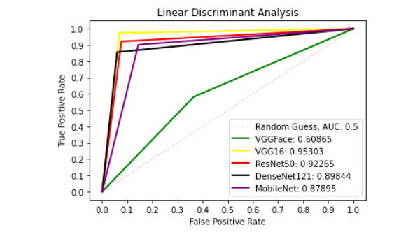
Figure 15. ROC curve with LDA comparing deep features using full liver images. ROC: Receiver operating characteristics; LDA: linear discriminant analysis.
We have seen so far the problem associated with patch liver images when used to detect steatosis within the hepatic liver cells. For example, one particular study[15], as presented in the literature section of this paper, successfully achieved 73% accuracy on binary classification problems; hepatic steatosis
Furthermore, as reported in the literature[42], hepatic steatosis was categorised into three; mild (with steatosis ranging between 5%-33%), moderate (with steatosis ranging between 33%-66%), severe (with steatosis above 66%) and normal for all those with less than 5% steatosis. By fine-tuning VGG16 and transforming the output layer into a binary classifier, each steatosis category was run against the healthy liver class, and the AUC in detecting mild, moderate, and severe steatosis were 0.71, 0.75 and 0.88, respectively. In terms of accuracy compared to the previous studies, we reported a highly improved detection of the steatosis within the hepatic liver cells with an accuracy of up to 92.99% using patch RGB images and with an AUC score of 0.9306. All these results are quite promising and has proved that Artificial Intelligence has the potential to assess fat within the liver organ. However, our subsequent experiment shows that using biopsied samples or patch images of the liver organ, some features are not seen by the deep learning algorithm. They get obscured and end up undetected. This is attributed to the tendency of missing the actual target during biopsy extraction due to sampling errors. This problem applies to patch extraction from the whole organ as well. Using the whole image of the organ presents an ultimate chance for the learning algorithm to screen all the pixels without missing a bit. Our result in this aspect achieved a near perfect detection performance of up to 99.63% and with an AUC score of 0.9958.
Computational consideration
For classification algorithms, speed and convergence are important considerations to make. At this point, we present a critical analysis of the classification algorithms considering the training efficiency in terms of the duration each algorithm takes to classify the features fed into it. This is important because one of the primary objectives of using AI to detect steatosis in the liver organs is the ability to execute a complex task that may take humans long duration; hours, days, months, etc., to complete. Therefore, it is critically important also to determine a specific algorithm that works best by finding the trade-off in terms of the accuracy and the execution time.
We begin by considering the results presented in Table 1, that is, the classification accuracies using the patch liver images. To be more precise, we start by considering the trade-offs using the SVM classifier. The result shows detection of the liver steatosis is 85.42% with the VGGFace features, and it takes 8.84 seconds as execution time. With VGG16 features, the classification is 90.72 % in 11.30 seconds, more accurate than with the VGGFace features but a bit longer execution time, though a marginal difference. The SVM + ResNet50 features achieved detection accuracy of 90.91% in 6.74 seconds, which obviously outperformed SVM + VGG16 features both in terms of accuracy and speed. The SVM + DenseNet121 and SVM + MobileNet features yielded detection accuracy of 88.83% and 72.54% while the execution times are 3.67 and 4.08 seconds, respectively.
The KNN + VGGFace and KNN + VGGa6 features yielded detection accuracies of 82.01% and 69.51%, while the respective execution times are 10.46 and 19.27 seconds, respectively. Here, the KNN worked better with the VGGFace features than with the VGG16 features. The KNN + ResNet50 and KNN + DenseNet121 features produced detection accuracies of 85.80% and 86.17%, while the respective execution times are 8.75 and 4.45 seconds, respectively. Lastly, the KNN + MobileNet features yielded a detection accuracy of 74.24% in 4.33 seconds. Using the KNN classifier, DenseNet121 features are the best in terms of accuracy and speed.
The LR + VGGFace and LR + VGG16 features achieved 86.55% and 90.53% accuracy, while the execution times were 2.06 and 3.38 seconds, respectively. The LR worked better with VGG16 features than with the VGGFace features. For the LR + ResNet50 and LR + DenseNet121 features, the detection accuracies are 92.99% and 90.53%, while the execution times are 1.58 and 0.84 seconds, respectively. The LR with ResNet50 features has outperformed all the combinations so far, including the LR + MobileNet features that achieved detection accuracy of 76.89% in 0.80 seconds.
It took the DT 18.18 and 15.81 seconds with the VGGFace and VGG16 features to yield 78.98 and 80.30 seconds, respectively. The DT + Resnet50 and DT + DenseNet121 features successfully achieved detection accuracy of 84.09% and 82.39% in 8.03 and 4.67 seconds respectively, while the DT + MobileNet features yielded detection accuracy of 65.72% in 3.25 seconds.
Finally, the LDA + VGGFace and LDA + VGG16 achieved detection accuracies of 68.37% and 88.26% in 12.02 and 15.38 seconds, respectively. The LDA with ResNet50 and DenseNet121 features achieved detection accuracy of 83.52% and 73.86% in 9.93 and 5.30 seconds, respectively, while with the MobileNet features, the detection accuracy of 60.04% in 5.96 seconds was achieved. In summary, using patch liver images, the ResNet50 features along with the LR provided the best trade-off, and Table 3 presents the summary of the times taken by each classification algorithm on each of the features.
Comparing computational efficiency (seconds) using full images
| Features | Classifiers | ||||
| SVM | KNN | LR | DT | LDA | |
| SVM: Support vector machine; KNN: K-nearest neighbour; LR: linear regression; DT: decision tree; LDA: linear discriminant analysis. | |||||
| VGGFace | 2.38 | 2.87 | 1.31 | 3.73 | 3.74 |
| VGG16 | 2.16 | 5.38 | 1.67 | 1.73 | 5.17 |
| ResNet50 | 2.48 | 2.78 | 0.47 | 1.61 | 2.93 |
| DenseNet121 | 0.39 | 1.17 | 0.28 | 0.82 | 2.02 |
| MobileNet | 0.55 | 1.95 | 0.29 | 1.42 | 2.57 |
In conclusion, we have presented the value and role of using machine learning to analyse the hepatic fat in liver images by applying deep learning techniques. Various deep learning models have been used along with classification algorithms for feature extraction and classification. One would have noticed that none of the deep learning models has been trained from scratch in the experiments we have reported. This is due to the lack of sufficient data for comprehensively training models. As a result, in our experiments, we have utilised transfer learning. The deep learning models used are the VGGFace, VGG16, ResNet50, DenseNet121 and MobileNet, and the classification algorithms are, the SVM, KNN, LR, DT and LDA.
The study shows that using deep learning to analyse hepatic steatosis prior to transplantation of the liver has the potential to minimise inter-observer variability and assessment biases. The experiments conducted show that the highest classification performance is obtained using ImageNet deep learning models combined with full liver images, achieving the accuracy of 99.63% using the SVM classifier. The computational for this classification is less than half a second on a standard laptop computer. The major advantages or strengths of using deep learning are the accuracy, efficiency, speed and non-invasive nature of the analysis compared to, for example, the standard method of using biopsy.
Despite the very promising nature of using deep learning for liver image classification reported in this study, limitations are observed, and they must be addressed. First, the amount of data is not sufficient. Therefore a large number of images is required to further improve the robustness of the analysis. Secondly, to improve upon this work further, the method must be benchmarked against a sufficiently large dataset that has been manually labelled. To our knowledge - aside from NORIS, which is of relatively small scale - such a dataset is not presently available in the public domain. Finally, a method of this nature must be extensively tested and verified using qualified surgeons and clinicians before one can realise its practical viability.
DECLARATIONS
Authors' contributions
Made substantial contributions to conception and design of the study and performed data analysis and interpretation: Ugail H, Wilson C
Undertook model development, experimentation and performed data analysis and interpretation: Abubakar A, Elmahmudi A
Performed data acquisition, as well as provided technical, and writing support: Thomson B
Availability of data and materials
Not applicable.
Financial support and sponsorship
We acknowledge funding for this research from UK Grow MedTech under the research project, POC 000135, "Liver organ quality assessment using photographic imaging analysis - LiQu".
Conflicts of interest
The authors declared that there are no conflicts of interest.
Ethical approval and consent to participate
Not applicable.
Consent for publication
Not applicable.
Copyright
© The Author(s) 2022.
REFERENCES
1. Ozturk A, Grajo JR, Gee MS, et al. Quantitative hepatic fat quantification in non-alcoholic fatty liver disease using ultrasound-based techniques: a review of literature and their diagnostic performance. Ultrasound Med Biol 2018;44:2461-75.
3. Schwimmer JB, Deutsch R, Kahen T, Lavine JE, Stanley C, Behling C. Prevalence of fatty liver in children and adolescents. Pediatrics 2006;118:1388-93.
4. Katsagoni CN, Papachristou E, Sidossis A, Sidossis L. Effects of dietary and lifestyle interventions on liver, clinical and metabolic parameters in children and adolescents with non-alcoholic fatty liver disease: a systematic review. Nutrients 2020;12:2864.
5. Croome KP, Lee DD, Croome S, et al. The impact of postreperfusion syndrome during liver transplantation using livers with significant macrosteatosis. Am J Transplant 2019;19:2550-9.
6. Jackson KR, Motter JD, Haugen CE, et al. Minimizing risks of liver transplantation with steatotic donor livers by preferred recipient matching. Transplantation 2020;104:1604-11.
7. Byra M, Han A, Boehringer AS, et al. Liver fat assessment in multiview sonography using transfer learning with convolutional neural networks. J of Ultrasound Medicine 2022;41:175-84.
8. Marcon F, Schlegel A, Bartlett DC, et al. Utilization of declined liver grafts yields comparable transplant outcomes and previous decline should not be a deterrent to graft use. Transplantation 2018;102:e211-8.
9. Cesaretti M, Brustia R, Goumard C, et al. Use of artificial intelligence as an innovative method for liver graft macrosteatosis assessment. Liver Transpl 2020;26:1224-32.
10. Mergental H, Laing RW, Kirkham AJ, et al. Transplantation of discarded livers following viability testing with normothermic machine perfusion. Nat Commun 2020;11:2939.
11. Schwenzer NF, Springer F, Schraml C, Stefan N, Machann J, Schick F. Non-invasive assessment and quantification of liver steatosis by ultrasound, computed tomography and magnetic resonance. J Hepatol 2009;51:433-45.
12. Taylor KJ, Gorelick FS, Rosenfield AT, Riely CA. Ultrasonography of alcoholic liver disease with histological correlation. Radiology 1981;141:157-61.
13. Meek DR, Mills PR, Gray HW, Duncan JG, Russell RI, McKillop JH. A comparison of computed tomography, ultrasound and scintigraphy in the diagnosis of alcoholic liver disease. Br J Radiol 1984;57:23-7.
14. Yersiz H, Lee C, Kaldas FM, et al. Assessment of hepatic steatosis by transplant surgeon and expert pathologist: a prospective, double-blind evaluation of 201 donor livers: assessment of steatosis in donor livers. Liver Transpl 2013;19:437-49.
15. Moccia S, Mattos LS, Patrini I, et al. Computer-assisted liver graft steatosis assessment via learning-based texture analysis. Int J Comput Assist Radiol Surg 2018;13:1357-67.
16. Abubakar A, Ugail H, Smith KM, Bukar AM, Elmahmudi A. Burns depth assessment using deep learning features. J Med Biol Eng 2020;40:923-33.
17. Wu X, Chen H, Wu X, Wu S, Huang J. Burn image recognition of medical images based on deep learning: from CNNs to advanced networks. Neural Process Lett 2021;53:2439-56.
18. Boumaraf S, Liu X, Zheng Z, Ma X, Ferkous C. A new transfer learning based approach to magnification dependent and independent classification of breast cancer in histopathological images. Biomedical Signal Processing and Control 2021;63:102192.
19. Rai R, Sisodia DS. Real-time data augmentation based transfer learning model for breast cancer diagnosis using histopathological images. In: Rizvanov AA, Singh BK, Ganasala P, editors. Advances in biomedical engineering and technology. Singapore: Springer; 2021. p. 473-88.
20. Minaee S, Kafieh R, Sonka M, Yazdani S, Jamalipour Soufi G. Deep-COVID: predicting COVID-19 from chest X-ray images using deep transfer learning. Med Image Anal 2020;65:101794.
21. Yoo SH, Geng H, Chiu TL, et al. Deep learning-based decision-tree classifier for COVID-19 diagnosis from chest X-ray imaging. Front Med (Lausanne) 2020;7:427.
22. Aslan MF, Unlersen MF, Sabanci K, Durdu A. CNN-based transfer learning-BiLSTM network: a novel approach for COVID-19 infection detection. Appl Soft Comput 2021;98:106912.
23. Pérez E, Reyes O, Ventura S. Convolutional neural networks for the automatic diagnosis of melanoma: an extensive experimental study. Medical Image Analysis 2021;67:101858.
24. Khan MA, Akram T, Zhang Y, Sharif M. Attributes based skin lesion detection and recognition: a mask RCNN and transfer learning-based deep learning framework. Pattern Recognition Letters 2021;143:58-66.
25. Reddy MS, Bhati C, Neil D, Mirza DF, Manas DM. National organ retrieval imaging system: results of the pilot study. Transpl Int 2008;21:1036-44.
26. Wu T, Gu X, Shao J, Zhou R, Li Z. Colour image segmentation based on a convex K-means approach. IET Image Processing 2021.
27. Ganesan P, Sathish BS, Leo Joseph LMI, Subramanian KM, Murugesan R. The impact of distance measures in K-means clustering algorithm for natural color images. In: Chiplunkar NN, Fukao T, editors. Advances in artificial intelligence and data engineering. Singapore: Springer; 2021. p. 947-63.
28. Abubakar A, Ugail H, Bukar AM. Noninvasive assessment and classification of human skin burns using images of Caucasian and African patients. J Electron Imag 2020;29:1.
29. Elmahmudi A, Ugail H. Experiments on deep face recognition using partial faces. 2018 International Conference on Cyberworlds (CW); 2018. p. 357-62.
30. Parkhi OM, Vedaldi A, Zisserman A. Deep face recognition. Available from: http://cis.csuohio.edu/sschung/CIS660/DeepFaceRecognition_parkhi15.pdf [Last accessed on 6 Jun 2022].
31. Simonyan K, Zisserman A. Very deep convolutional networks for large-scale image recognition. arXiv preprint arXiv 2014.
32. He K, Zhang X, Ren S, Sun J. Deep residual learning for image recognition. Proceedings of the IEEE Conference on Computer Vision and Pattern Recognition; 2016. p. 770-778. Available from: https://openaccess.thecvf.com/content_cvpr_2016/papers/He_Deep_Residual_Learning_CVPR_2016_paper.pdf [Last accessed on 6 Jun 2022].
33. Huang G, Liu Z, van der Maaten L, Weinberger KQ. Densely connected convolutional networks. Proceedings of the IEEE Conference on Computer Vision and Pattern Recognition; 2017. p. 4700-08. Available from: https://openaccess.thecvf.com/content_cvpr_2017/papers/Huang_Densely_Connected_Convolutional_CVPR_2017_paper.pdf [Last accessed on 6 Jun 2022].
34. Howard AG, Zhu M, Chen B, et al. Mobilenets: efficient convolutional neural networks for mobile vision applications. arXiv preprint arXiv 2017.
35. Deng J, Dong W, Socher R, Li LJ, Li K, Dept LFF. Imagenet: a large-scale hierarchical image database. Proc. CVPR 2009. p. 248-55.
36. Gunn SR. Support vector machines for classification and regression. ISIS Technical Report; 1998. p. 5-16. Available from: https://see.xidian.edu.cn/faculty/chzheng/bishe/indexfiles/new_folder/svm.pdf [Last accessed on 6 Jun 2022].
37. Jiang L, Cai Z, Wang D, Jiang S. Survey of improving k-nearest-neighbor for classification. Fourth International Conference on Fuzzy Systems and Knowledge Discovery (FSKD 2007); 2007. p. 679-83.
38. Biosa G, Giurghita D, Alladio E, Vincenti M, Neocleous T. Evaluation of forensic data using logistic regression-based classification methods and an R shiny implementation. Front Chem 2020;8:738.
39. Dreiseitl S, Ohno-machado L. Logistic regression and artificial neural network classification models: a methodology review. Journal of Biomedical Informatics 2002;35:352-9.
40. Gyamfi KS, Brusey J, Hunt A, Gaura E. Linear classifier design under heteroscedasticity in linear discriminant analysis. Expert Systems with Applications 2017;79:44-52.
41. Byra M, Styczynski G, Szmigielski C, et al. Transfer learning with deep convolutional neural network for liver steatosis assessment in ultrasound images. Int J Comput Assist Radiol Surg 2018;13:1895-903.
Cite This Article
Export citation file: BibTeX | RIS
OAE Style
Ugail H, Abubakar A, Elmahmudi A, Wilson C, Thomson B. The use of pre-trained deep learning models for the photographic assessment of donor livers for transplantation. Art Int Surg 2022;2:101-19. http://dx.doi.org/10.20517/ais.2022.06
AMA Style
Ugail H, Abubakar A, Elmahmudi A, Wilson C, Thomson B. The use of pre-trained deep learning models for the photographic assessment of donor livers for transplantation. Artificial Intelligence Surgery. 2022; 2(2): 101-19. http://dx.doi.org/10.20517/ais.2022.06
Chicago/Turabian Style
Ugail, Hassan, Aliyu Abubakar, Ali Elmahmudi, Colin Wilson, Brian Thomson. 2022. "The use of pre-trained deep learning models for the photographic assessment of donor livers for transplantation" Artificial Intelligence Surgery. 2, no.2: 101-19. http://dx.doi.org/10.20517/ais.2022.06
ACS Style
Ugail, H.; Abubakar A.; Elmahmudi A.; Wilson C.; Thomson B. The use of pre-trained deep learning models for the photographic assessment of donor livers for transplantation. Art. Int. Surg. 2022, 2, 101-19. http://dx.doi.org/10.20517/ais.2022.06
About This Article
Copyright

Data & Comments
Data


 Cite This Article 11 clicks

 Like This Article 6
likes
Like This Article 6
likes


Comments
Comments must be written in English. Spam, offensive content, impersonation, and private information will not be permitted. If any comment is reported and identified as inappropriate content by OAE staff, the comment will be removed without notice. If you have any queries or need any help, please contact us at support@oaepublish.com.